Take a bearing, don't estimate - Update

I believe forecasting software development using the Monte Carlo method is even easier than I thought. In my previous article I used averages of past cycle times to come up with an idea of how much effort future tasks would take.

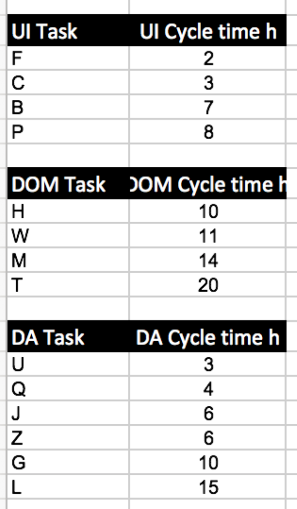
This was my basic data set: a log of cycle times of 14 tasks already accomplished, each belonging to some category.

As a very simple way to calculate an expected effort for future tasks A (UI), K (DOM), E (DA), V (DOM), R (DA), X (UI) I suggested to use the average task cycle time per category. This would lead to A (5h), K (13.75h), E (7.33h), V (13.75h), R (7.33h), X (5h) = 52.17h in total.

That’s easily done. No problem. And if you just have a pocket calculator around you might want to go with this.

But if you happen to have Excel handy, then you should try do not calculate the expected effort, but do a simulation. I did that using the Monte Carlo method.

Today, though, I’m not satisfied anymore with my approach how I used the Monte Carlo method. I had some qualms already while I wrote the article. I wanted to use the real distribution of the data points to base the simulation on - but somehow didn’t see how to do it. So I again used the average category values with some random variation.

But now I know better, I guess. Had to let it sink in, take a shower, go for a walk… ;-)

Here’s my new approach. Hope you’ll find that even simpler.

Using the Category Distributions

First group the data points according to their categories:

As you can see, their distributions differ somewhat:

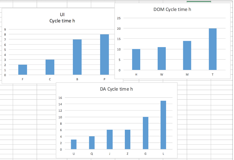
This is what should show up in the simulation. The aggregated distribution should mirror the de facto skew of the original distributions matching future task categories.

An even easier Monte Carlo simulation

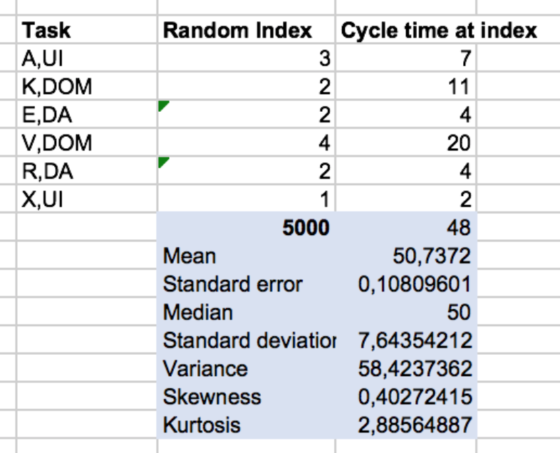
As it turns out this is very simply done: for each future task I just have to pick a random task from its category. That’s it. The random index lies in the range of 1..n with UI(n=4), DOM(n=4), DA(n=6).  As long as the random indexes are evenly distributed the cycle times picked will follow the original distribution. Why didn’t I think about that earlier?

The total expected cycle time of course still is the sum of the randomly calculated cycle times for each of the future tasks. But no averages are used anymore, no standard deviation is added/subtracted. It’s just a plain random picking of logged values.

After 5000 runs of this calculation the resulting distribution looks like this:

Compared to the previous approach it’s not normally distributed anymore which is great. To me that suggests it’s truly mirroring the underlying distributions. As you can see above those seem to be skewed somewhat to lower numbers - which is the case for the simulation, too.

Not using averages now gives a different picture of expected efforts. The average of the total over all simulation runs is 50.73h which is somewhat lower than before (52.31h) - as expected. But more importantly, when you look at the curve, you see that the 90% threshold is now higher: 60.82h compared to 58.45h before! The same is true for the 80% threshold, but not the 66% threshold. That’s somewhat unexpected, isn’t it? But I like it ;-)

If you want a 0.9 probability for a total expected effort for six new tasks with certain categories you should plan a budget of 60.82 hours. This is some 20% more than the average. Before the difference was only 11%.

To me this sounds much more reasonable. I’m glad I gave it another thought. The simulation is now easier, more straightforward, and the results are matching my intuition better.