Don’t be wrong on average! - Software delivery forecasting using simulation
Let’s be honest: estimating software development effort does not work and is a constant pain in the ass for developers.
It does not work because the real time needed to deliver estimated work items is off by more than 10% in 90% of the cases. And it’s always off to the wrong side: it never takes less time but always takes longer.
And it’s a pain in the ass because everyone knows it’s wrong and stress will ensue and whatever number the developer tells will not be accepted right away but will be haggled over.
There’s only one thing that can be done about it: stop software estimation now! Don’t kid yourself any longer.
But what then? The questions won’t stop: „When will it be done?“, „How long will it take to finish these work items?“
As much as I’d like to get into a working mode where those questions wouldn’t be asked again, I have to acknowledge that’s too much of a cultural change to ask for. So, how to answer them without estimation, without stress?
I think the only way is to resort to facts. Finally. Facts and statistics. Don’t dream up arbitrary numbers any longer. Instead look at what’s there.
A simplistic approach to forecasting a delivery date
The other day I read „You don’t need story points“ by Neil Killick. The headline caught my eye and I like the basic idea:
- Stop estimating story points, instead categorize work items according to t-shirt sizes (S, M, L,…) upon acceptance to your backlog.
- As long as work items sit in the backlog they may be of different size, but once you really start working on them you slice them into S-sized work items.
- Count how many S-sized work items you deliver per time period (e.g. week or sprint)
- Calculate averages: How many S-sized work items do M- and L-sized ones get sliced into on average? How many S-sized work items are delivered on average per time period (throughput)?
Neil Killick gives an example:
- Assume a backlog with work items of this size: 11 S, 35 M, 20 L.
- Assume average slicing ratios like this: 1 M = 5 S, 1 L = 12 S.
This backlog then represents 11 + 35*5 + 20*12 = 426 S-sized work items.
The example in the article unfortunately ends here. No answer is given to the question „How long will it take to deliver all that’s sitting in the backlog?“
So let me extend the example with one more assumption:
- Assume an average throughput of 7 work items per time period (e.g. week, sprint).
The forecast then is 426 / 7 = 60,85 time periods.
Not bad, isn’t it? No estimation effort. No abstract story points, but a tangible number in terms of days or weeks or sprints. You can enter a delivery date into the calendar right away. Simple calculation saved the day.
The only „divination“ happening is the categorization. But compared to story point estimation that’s easy. And, hey, it doesn’t even have to be that accurate, because in the end what counts is counting. That’s even easier.
Developers just need to count the conversion rates from M and L to S, and the number of S-sized work items delivered per time period. That can easily be done by hand, or maybe some work item tracking tool can help with it.
The story could end here. Embrace Neil Killick’s recommendation and life will be good as a developer once more.
And maybe you really should start out like that. It won’t reduce the frustration and the stress in the end, but at least the burden of estimation is gone. That already might be a worthwhile benefit.
If you stop reading here I don’t blame you. Start your new #noestimates habit now!
Avoid the single number!
You’re still reading on? You’re not entirely convinced it’s that simple to escape the estimation trap and you want to really avoid stress? Great, then let me tell you why after initial enthusiasm about the article I was disappointed at the end:
I’ve long since lost the belief in a simple and single number as the answer to the notorious question „How long will it take?“
Expecting a single number and telling a single number is the fundamental flaw behind all software estimation I see in teams. My guess is, developers know that intuitively - but don’t know what to do about it. And managers… I don’t know if they know. But they should. They even should be the first to refuse such a simplification.
There are several problems with the single number answer:
- The single number does not mirror reality. Reality is messy, it’s full of uncertainty. There is no such thing as delivering in exactly 60,85 time periods. It will take less time or more time. But how muss less or more? No range is given for the delivery time. That’s especially bad since the difference between number and reality in the end will not be negligible. It will not be just 5% off. By ignoring this reality stress, pressure, conflicts, blame are guaranteed to follow.
- Since the single number does not transport uncertainty it also does not convey risk. A decision maker cannot match the number to his/her risk attitude. Some feel lucky, some are risk averse. No way to tell what the „risk level“ of a single number is. Or if one should be assumed then it’s a 50:50 change of success because the single number just represents some average. But is that really what a decision maker want’s to do: play a game with just a 0.5 probability to win?
- When playing Roulette and betting on Red or Black you end up neither winning or losing in the long run. Because if you lose your bet in one round you’ll win in a later round and the other way around. So just stay in the game long enough to go home even. This might be difficult to endure, but the odds are in your favour. The same cannot be said for bets in software development, though. What is said about casinos - „The casino always wins“ - is true here, too, and can be phrased like „The team always loses“. It always loses when betting on a single number, because there is no winning. There is no early delivery next time to compensate for late delivery this time. The simple reason for that: Parkinson’s law. Once there is a date set for delivery the time until then will always be used up. There’s no incentive for delivering early. And there’s no penalty for taking as long as scheduled. However, delivering late is always equal to losing. You’re losing trust, you’re losing money. Sometimes there’s even a penalty fee for each day a delivery is late. But there’s hardly ever a bonus for delivering early; and if there where it’s very hard to get it. Betting on the single number in software development thus resembles throwing a coin and not losing any money on heads, but always losing on tails. Would you play such a game?
- Finally, even if a single number is given with doubts and pleas for caution added to document one’s consciousness about uncertainty it’s taken as a single number. Any attachments are stripped off immediately by the receiver. The single number becomes a fact, a promise.
When a single number is asked for, the answer is an average by default. „How long do you think it will take you to implement this?“ The developer then rummages around in his memory and comes up with a gut feeling. In this feeling all experience is condensed into… an average. „It feels like it should take 3 days,“ might be the answer. But 3 days is not the maximum and not the minimum. Neither are maximum or minimum efforts remembered exactly, nor is there any incentive to tell them if they were known. And why should a „similar task“ take the minimum or maximum amount of time anyway? It’s more likely to take time around the average.
An average is also the result if several developers are asked. One’s gut feelings are 2 days, another one’s are 5 days. So what’s the single number given? It will be around 3.5 days - except when there is a very compelling argument that one of them is far off with his or her gut feeling.
In Neil Killick’s approach averages are even used explicitly. There is the average slicing rate for M and L work items, there is the average throughput.
One uncertainty is added to another uncertainty and even a third uncertainty is heaped on top of this. This will hardly lead to satisfying results.
And remember: As soon as any single number is given it’s taken as gospel and must be adhered to.
So there is only a single solution to the single number problem: Don’t!
Don’t ever give single numbers (averages) as answers to questions where considerable uncertainty is involved.
Distributions to the rescue!
Whoever asks the unholy question wants a simple answer. As simple as possible, but as realistic as necessary. A single number won’t do, but a list of numbers will.
Let’s take the 5 S-items per M-item as an example. It’s a single number, the average slicing rate. But doesn’t it make a difference whether it’s the average of (1,2,3,4,5,6,7,8,9) or (1,1,1,2,7,8,8,8,9)?
Here’s the proof:
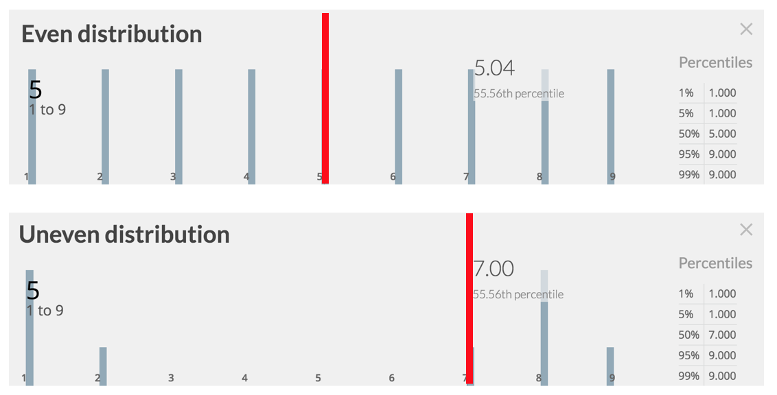
Look at the bars and look at the numbers. The obvious difference is in the shape of the histogram: in the first one all bars are of equal length, not so in the second one. But then there is another, more subtle difference: in the second distribution the mean is not equal to the median.
Let me make this more tangible for you: in the first distribution you have a roughly 50% chance that an M-item will be sliced into 5 or less S-items. In the second distribution, though, the roughly 50% chance lies not with 5 - because there is no 5 -, but with 7.
Don’t you think that could be of some informative value to a decision maker?
A distribution is a range of values with frequencies and probabilities attached. Check out the second list of values:
- a list of 9 values ranging from 1 to 9
- the frequencies are: 3x1, 1x2, 1x7, 3x8, 1x9
- the probabilities are for example: a 0.33 (33%) chance of slicing a M-item into just 1 S-item or a 0.55 (55%) chance for up to 7 S-items.
Or if you like, turn chance around into risk. Distributions make explicit the risk you’re taking up when you pick a single number. For example a 33% chance equals a 77% risk.
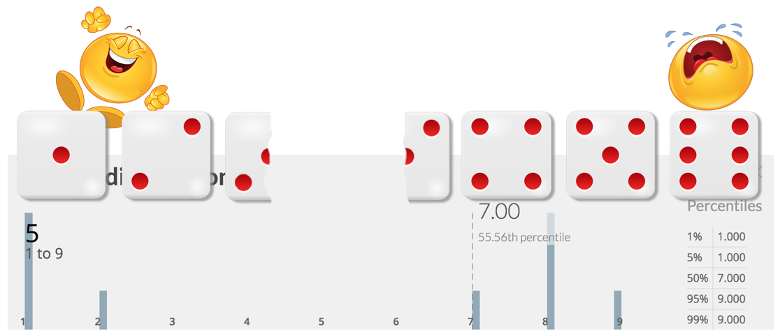
If it’s hard for you to „feel“ risk think of rolling a die. What’s the risk of not slicing a M-item into 5 S-items?
With the first distribution you’d win when rolling 1, 2 or 3, you lose when rolling 4, 5, or 6.
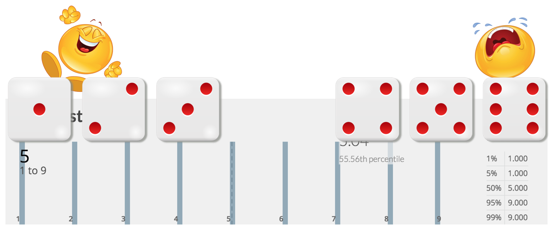
But with the second distribution if you’d bet on the average - or mean - you’d only win when rolling a 1 or 2 (or every second time you roll a 3).
Do you still think this is a game anyone would play regularly if thousands of dollars are at stake? And remember: There is no real gain in case of early delivery - but there’s always a penalty of some sort upon late delivery.
A distribution like this is not only fact based but also a gauge for risk. A decision maker sees how risk develops over time - early delivery date = higher risk, later delivery date = lower risk - and can make an informed decision according to his/her risk attitude.
What would you go for? What should the odds be if you’d had to promise somebody on time delivery? Would 50% be enough or would you want 83% or 95% „certainty“?
And remember: Any such distribution is based on a particular context in the past. Its forecasting capability is limited. If things have changed since the historical data has been compiled - e.g. somebody left the team, the focus of development has shifted, experience has been gained, infrastructure changed, new technologies where introduced - the future will likely look different. Even just 1% risk means there is no certainty. Things can still take longer, much longer. (And rarely if ever they take less time than promised.)
That means: You constantly need to update your distributions. Never stop measuring, never stop recalculating, never stop watching how the odds evolve. Instead of a single estimation or forecast a stream of forecasts needs to be produced.
Calculating with distributions
If distributions are the answer to the question „When will it be done?“ how then to use them in a scenario like the above?
Here’s how I’d do it these days:

Don’t despair! This just looks complicated at first sight. Let me take you on a tour of this model which is based on Monte Carlo simulations. It’s done with getguesstimate.com (GitHub repo) and you can play around with it here. You’ll see it’s actually straightforward and simple.
Every box contains a value like in the cells of an Excel sheet. Either it’s a fixed value or it’s a calculated value. Here are examples of both:
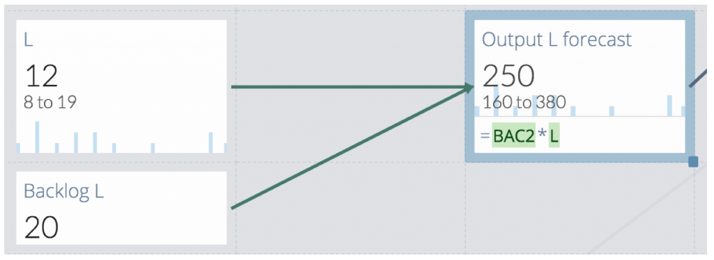
Value „Backlog L“ is the number of backlog items of size L. It’s a single value as given by Neil Killick.
Value „L“ on the other hand is a distribution. It’s given as a list of numbers with a certain average as given by Neil Killick. Here’s a close-up of the distribution and an excerpt from the underlying numbers.
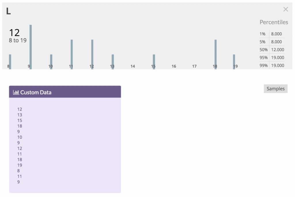
I chose the numbers to mimic what I think would be a realistic distribution with the average given in the example. As you can see it’s not a normal distribution (no bell shape). It’s skewed to the left, and there is a second, smaller hump to the right. The most likely number of S-items to slice an M-item into is 9 - but unfortunately that’s not a very likely result to expect when slicing.
Developers are pretty good at assessing backlog items as S or M or L. But, well, sometimes they ere. That’s human. Sometimes an M-item really is an L-item, and sometimes an L-item really is an M-item. That’s how life is.
In the example what is certain is how many items in each category are in the backlog. What’s not certain is, how many S-items that ultimately will lead to.
This kind of uncertainty must not be glossed over by using an average! Instead a distribution should be calculated from factual data. That’s what „Output L forecast“ does. It multiplies the number of L items with the distribution of S-items per L-item to arrive at a distribution of S-items for the current backlog’s L-items.
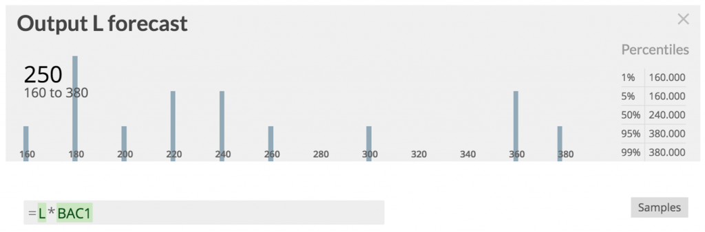
On average 250 S-items might be sliced from 20 L-items. But how many will it be for the actual 20 items in the backlog right now? The average is only a statement about many trials. The distribution, however, shows nicely what number to expect with what kind of risk.
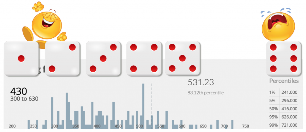
The same is done for the M-items. And then the distributions for the S-items from M- und L-items plus the S-items in the backlog are combined into a distribution for the total number of S-items to expect, the „Backlog forecast“:
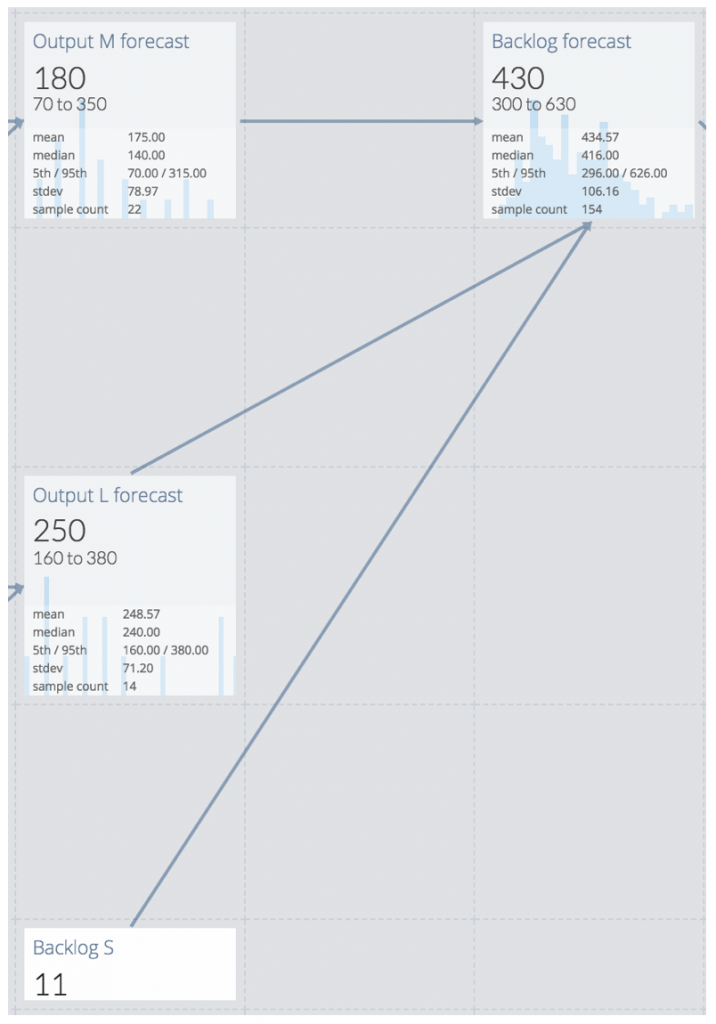
Where Neil Killick ended up with just a single number of „exactly“ 426 items, the model show’s the actual range of values is pretty wide: from 300 to 630.
And again the question is: How lucky do you feel? Would you go with 426 (or 430) like Neil Killick suggests? That would be like tossing a coin. Or would you be more inclined to roll a dice and win with any number except for when you roll a 6? For that you’d have to go for at least 530 S-items at the 83rd percentile.
But what does that mean in terms of a delivery date? Throughput has to be taken into account - which of course has to be represented with a distribution, not a single number.
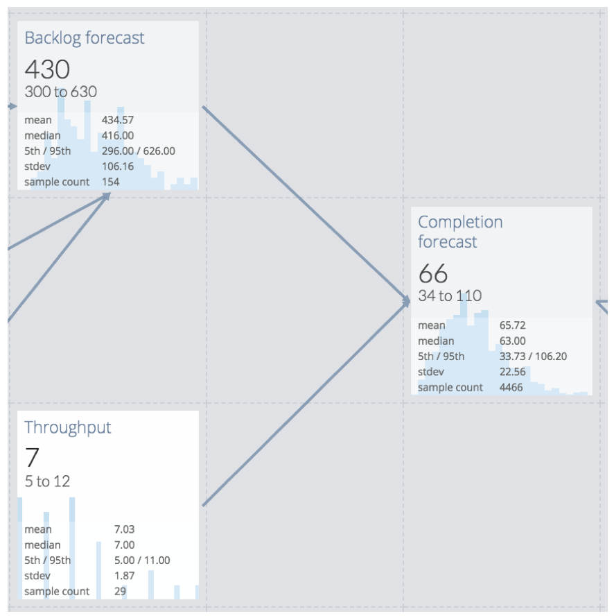
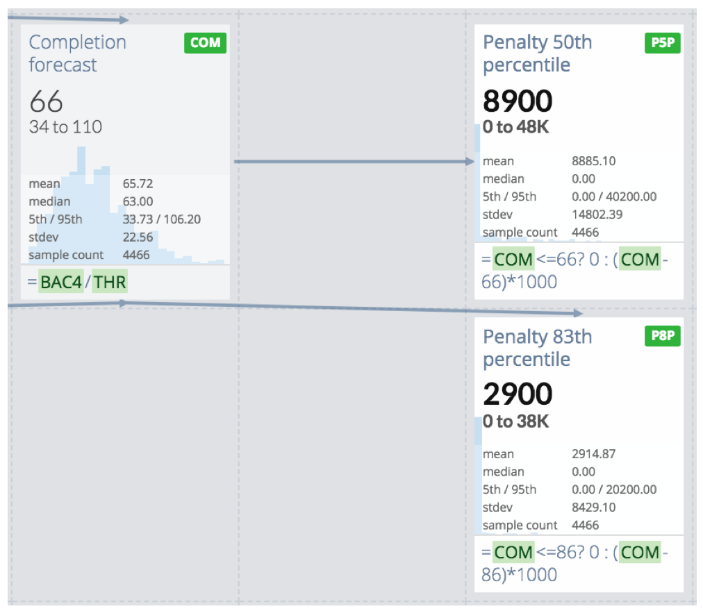
Finally the „Completion forecast“ yields a time span when delivery of the example backlog can be expected:
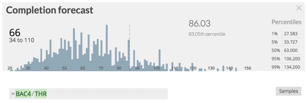
It’s not just in 66 time periods, but depends on a lot of factors. It ranges from 34 to 110 time periods - and if you’d want to play a pretty safe game (only loose when you roll a 6) you’d go for 86 time periods.
So much for an alternative view on Nick Killick’s example. In the end he, too, says „You can also plug your numbers into a Monte Carlo simulation tool“ - but who actually reads that far? I almost did not. Also he acknowledges uncertainty by saying „The volatility in your delivery rate can be measured using one or two standard deviations of the delivery count numbers you’ve been recording.“ But that, too, is rather at the end of the article and is not bolstered by any calculations or examples. (In addition I find visualizations much more tangible than just numbers.) Thus my guess is, hardly anybody will follow these suggestions. And so his advice to let go of story points is still in the realm of the single number with all its problems.
But as you can see, calculating with distributions isn’t hard at all. Why resort to single numbers when you can retain all the data fidelity you have until the end?
So let’s take the example one step further? What about a penalty for late delivery? If you deliver on time all’s well. However if you deliver late you have to pay, e.g. 1000€ per time period you’re beyond the committed delivery date.
What can you expect to pay? Here’s a forecast for that:
The top cell on the right side shows the penalty distribution if you’d commit to the average of 66 time periods. The bottom cell on the right shows the penalty distribution for 86 time periods.
The average penalty might not differ that much, so you feel inclined to bet on the 66 time periods. But when you look closer, you might want to reconsider:
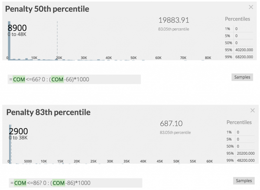
With the 66 time periods you’ll pay up to 20,000€ in 83% of the cases, but with 86 time periods it’s less than 700€. Not to speak of the stress when delivering late.
This underlines the asymmetry between delivering on time or even before and delivering late. Note the use of the ternary operator in the cells’ definitions for an expression of that.
Summary
Yes, give up story point estimation. But don’t fall for the „flaw of averages“! I recommend reading the like named book by Sam L. Savage. Also you should study „When will it be done?“ by Daniel Vacanti. It goes beyond calculating with distributions by talking about the process which may lead to useful numbers to be used in such calculations in the first place.
Check out getguesstimate.com to become familiar with using distributions instead of single values in calculations. Also you can learn about how to use Excel for these kind of calculations at SIPmath.org.
The main challenge now lies in getting your hands on real numbers. Forecasting is about counting. You need relevant collections of measurements to derive meaningful distributions from.
But that should be simpler and less stressful than ongoing demands for unfounded estimates. And ultimately it will invert the burden of producing an answer to the question „When will it be done?“ Because with historical data fed into a model like shown here, whoever is asking the question will be able to answer it for him-/herself.